NBA Team Projection Models: Intro & Test Data


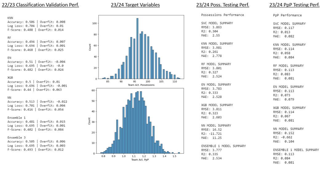
Our NBA team models are our oldest ongoing implementation, and we continue to iterate on them each year. For the 21/22 and 22/23 seasons, we utilized classification models based on team-level performance metrics and betting market data to arrive at the final win and cover probability estimates. For the 23/24 season, we experimented with moving our team-level algorithm to a regression-based approach centered around fundamental play-by-play data, and fit separate models for the two components of team points scored - game pace and points per possession (PpP). A few performance metrics for both approaches are shown below.
Our introduction of player prop models as well as game pace estimates also allowed us to generate an entirely new set of team predictions based on player-level data for the first time in 23/24. The NBA player model takes each player's net contribution per 100 possessions on both offense and defense, weights it for his minutes, and then sums the total to get an idea of each team's overall strength on both offense and defense. We found this approach to be the most effective in capturing daily rotation nuances in a sport where "load management" has become the norm, and thus it will be our main predictive team model for the 24/25 season.
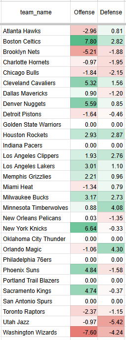
An example from a typical night during the season is shown below, with each team’s offensive and defensive points scored/allowed above the league average per 100 possessions. The higher the values for each, the better, hence the teams with the best record tend to have the highest total values across offense and defense. The contributions per 100 possessions are then scaled based on the projected pace of the game that day. To arrive at a point total estimate, Team A's offensive strength (measured in points scored above the league average per 100 possessions) is netted against Team B's defensive strength (measured in points allowed below the league average per 100 possessions). The same process is applied to Team B's offense and Team A's defensive totals. From there, we can infer a fair points spread on a neutral court.
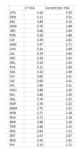
We then give the home team a points boost vs the spread based on 25,000 games to see how much they outperform vs a baseline expectation when playing at home. We then re-center each team's advantage to the league average to account for the relative decline in home court advantages in recent years. The long-term and current HCAs for each team are shown in the table below. This is not a perfect method, as a city's interest can ebb and flow based on how good or bad their team is, but it is the best we can do without inserting discretionary judgments. Unsurprisingly, the high altitude teams have had the biggest advantage over 10+ years of games.
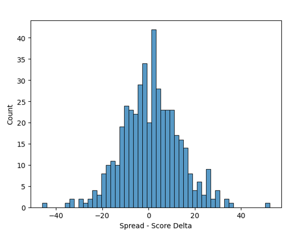
Once we have point totals and a home-court advantage estimate, we can make a final fair home spread estimate of (away projected score - home projected score - home court advantage). The final step is to convert these values to a probability to compare them with the odds-implied probabilities. Fortunately for us, spreads vs final results are normally distributed (histogram shown below), making the calculation trivial. By simply comparing the fair spread to the actual spread and providing the long-term standard deviation between projected spreads and outcomes, we can arrive at a solid estimate of a team's cover probability using the Gaussian CDF. The same process (with the home court advantage removed) is used to calculate over/under edges.

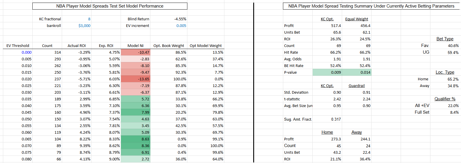
Player-Level Spreads
Model Test Performance Summary